Function transformations: new and old
This is one of the most annoying things to teach in any functions-based class: Supposing $a, b > 0$, why does the transformation $y=f(x-a)+b$ move the graph of $f$ to the right by $a$ and up by $b$, even though the signs are different? Why does the thing that's happening horizontally work “backwards” from the thing that's happening vertically? Prompted by a nice activity from Matt Enlow, I finally have an explanation that feels persuasive. I road-tested this with my “Functions Modeling Change” class this week, and I now am excited to share it more broadly.
The setup
So let's say that we have an original function $y=f(x)$ and a new function $y=g(x)$ that is some transformation of $f$. The key to this explanation is that those $y$'s and $x$'s are actually not the same! I am instead going to label them as follows1:
- An input to $f$ is called $\textcolor{red}{\text{old }x}$.
- An output of $f$ is called $\textcolor{red}{\text{old }y}$. In particular, $\textcolor{red}{\text{old }y} = f(\textcolor{red}{\text{old }x})$.
- An input to $g$ is called $\textcolor{blue}{\text{new }x}$.
- An output of $g$ is called $\textcolor{blue}{\text{new }y}$. In particular, $\textcolor{blue}{\text{new }y} = g(\textcolor{blue}{\text{new }x})$.
And yes, I am going to use those colors throughout this blog; in class I used two different color whiteboard markers.
Old and new labels in action
Let's look at a concrete example to see what this labeling wins us. Suppose that
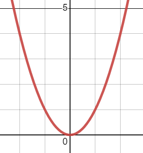
In the illustration below, I've chosen $f(x) = x^2$ just for concreteness, but the following will work with any choice of $f$.
| Old $f$ | New $g$ |
|---|---|
 |
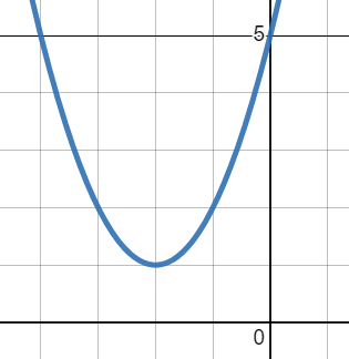 |
Let's apply our labels. The $y$ in $y = g(x) = f(x+2) +1$ is in fact a $\textcolor{blue}{\text{new }y}$, and the $x$ that's in the input of $g$ is in fact a $\textcolor{blue}{\text{new }x}$. The key thing to notice is that the $x$ inside the argument of $f$ is the same $x$ that's an input of $g$, so it also gets the $\textcolor{blue}{\text{new }x}$ label:
So now grab the entire argument of $f$ – the entire input of $f$ – and label it as $\textcolor{red}{\text{old }x}$:
This says that if you knew the $\textcolor{blue}{\text{new }x}$, you could add 2 to get the $\textcolor{red}{\text{old }x}$ – in other words, $\textcolor{red}{\text{old }x}$'s are 2 to the right of $\textcolor{blue}{\text{new }x}$'s. Equivalently, if you knew the $\textcolor{red}{\text{old }x}$ and wanted the $\textcolor{blue}{\text{new }x}$, you would have to subtract 2 – that is,
In other words, $\textcolor{blue}{\text{new }x}$'s are 2 to the left of $\textcolor{red}{\text{old }x}$'s.
Now that we've thought about $x$'s, let's think about $y$'s. Remember that $g(\textcolor{blue}{\text{new }x})$ = $\textcolor{blue}{\text{new }y}$, and $f(\textcolor{red}{\text{old }x})=\textcolor{red}{\text{old }y}$:
This says that if you knew the $\textcolor{red}{\text{old }y}$, you could add 1 to get the $\textcolor{blue}{\text{new }y}$ – in other words, $\textcolor{blue}{\text{new }y}$'s are 1 up from $\textcolor{red}{\text{old }y}$'s. Equivalently, if you knew the $\textcolor{blue}{\text{new }y}$ and wanted the $\textcolor{red}{\text{old }y}$, you would have to subtract 1 – that is,
In other words, $\textcolor{red}{\text{old }y}$'s are 1 down from $\textcolor{blue}{\text{new }y}$'s.
Here's the punchline: Subtracting from $x$ inside the argument of the original function is something you do to $\textcolor{blue}{\text{new }x}$. Adding to the output of $f$ is something you do to $\textcolor{red}{\text{old }y}$. This is why these two things behave in the opposite directions!
Rule of Four
I am a big fan of the idea that we can always represent functions in any of Four different ways:
- Verbally: describing a function or its context using human words
- Algebraically: using function notation, equations, and symbols
- Graphically: drawing graphs on the Cartesian plane
- Numerically: producing tables of values
The above explanation relies pretty heavily on algebraic and graphical representations of these functions; it's nice to also consider numerical representations. Here is a table of some easily-clockable points on $f(x) = x^2$:
(Notice the “old” labels on $x$ and $y$.)
Using the relationships $\textcolor{red}{\text{old }x} - 2 = \textcolor{blue}{\text{new }x}$ and $\textcolor{red}{\text{old }y} + 1 = \textcolor{blue}{\text{new }y}$, we can produce the following table of corresponding points on $g(x) = f(x+2) + 1$:
I found that having students work through modifying the old table to produce the new table was really persuasive.
Benefits and hurdles
What I really like about this argument is that it illustrates that left vs. right and up vs. down are a matter of perspective. Sure, $f(x-2)$ produces a new graph who's 2 to the right of original $f$, but equivalently, original $f$ is 2 to the left of the new graph. Sure, $f(x) - 3$ produces a new graph who's 3 down from original $f$, but equivalently, original $f$ is 3 up from the new graph.
Another thing I really like about this argument is that it emphasizes what you might call the Fundamental Principle of Functions: functions relate inputs to outputs. A key idea in the above argument is that $\textcolor{blue}{\text{new }y} = g(\textcolor{blue}{\text{new }x})$ – that is, that $\textcolor{blue}{\text{new }y}$ really does come from applying the function $g$ to the input $\textcolor{blue}{\text{new }x}$.
I think the biggest conceptual hurdle – based on running this by one class of students, so take this with an appropriately-sized nugget of salt – is that we must relabel the entire argument of $f$ as $\textcolor{red}{\text{old }x}$. This is somehow crucial, because it establishes the relationship between $\textcolor{red}{\text{old }x}$ and $\textcolor{blue}{\text{new }x}$, and it's also tricky. It's especially tricky if you are not doing a horizontal transformation. For instance, consider $y=g(x) = f(x) - 3$; with labels, this becomes $\textcolor{blue}{\text{new }y} = g(\textcolor{blue}{\text{new }x}) = f(\textcolor{blue}{\text{new }x}) - 3 $. It is tricky to notice that since nothing has happened to $\textcolor{blue}{\text{new }x}$ inside the argument of $f$, that $\textcolor{red}{\text{old }x} = \textcolor{blue}{\text{new }x}$ – that is, that $\textcolor{blue}{\text{new }x}$ and $\textcolor{red}{\text{old }x}$ are the same.
Exercise
Use new and old labels to convince yourself why $2f(x)$ is a vertical stretch and $f(2x)$ is a horizontal compression.
-
I considered using subscripts here – $x_\text{old}$, $y_\text{new}$, etc. – but ultimately decided against them on the grounds that my students hate subscripts, lol. ↩