
Section 3.2 The analytic formulation of the problem

In order to discuss intelligently the problem of the brachistochrone we should first deduce for ourselves the integral which represents the time required by a particle to fall under the action of gravity down an arbitrarily chosen curve joining two fixed points 1 and 2. It is agreed that the initial velocity \(v_1\) at the point 1 is given in advance, and that the particle is to fall without friction on the curve and without resistance in the surrounding medium. If the effects of friction or a resisting medium are to be taken into account the brachistochrone problem becomes a much more complicated one.

Activity 3.2.1.

I'm hiding the diagram included in the textbook under a little foldy thing. I encourage you to draw your own diagram first, based on the instructions in the next paragraph, and then compare your diagram to the one in the book. (This will actually help you make sense of the book's diagram when you see it, because there's some things that aren't super clear.) Label the following:

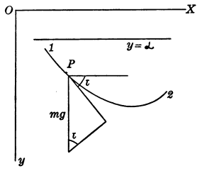
  • the curve of descent \(C\) connecting point 1 and point 2;

  • a moving particle \(P\) on the curve \(C\text{;}\)

  • the distance \(s\) that the point \(P\) has actually traveled so far;

  • a tangent line to the curve \(C\) at the point \(P\text{;}\)

  • the vertical and horizontal components of that tangent line;

  • the angle \(\tau\) between the horizontal and the tangent line; and

  • the downward force of gravity \(mg\text{.}\)

Solution
Diagram of a point moving along a curve under the force of gravity.
Figure 3.2.1.

Let \(m\) be the mass of the moving particle \(P\) in Figure 3.2.1 and \(s\) the distance through which it has fallen from the point 1 along the curve of descent \(C\) in the time \(t\text{.}\) In order to make our analysis more convenient we may take the positive \(y\)-axis vertically downward, as shown in the figure.

The vertical force of gravity acting upon \(P\) is the product of the mass \(m\) by the gravitational acceleration \(g\text{,}\) and the only force acting upon \(P\) in the direction of the tangent line to the curve is the projection \(mg \sin \tau\) of this vertical gravitational force upon that line. But the force along the tangent may also be computed as the product \(m \frac{d^2s}{dt^2}\) of the mass of the particle by its acceleration along the curve. Equating these two values we find the equation

\begin{equation*} \frac{d^2s}{dt^2} = g \sin \tau = g \frac{dy}{ds}, \end{equation*}

in which a common factor \(m\) has been discarded and use has been made of the well-known calculus formula \(\sin \tau = \frac{dy}{ds}\text{.}\)

Activity 3.2.2.

That's not a well-known formula to me! Draw yourself a little triangle with angle \(\tau\) and sides \(\Delta s\) and \(\Delta y\text{.}\) Use this to conclude \(\sin \tau = \frac{dy}{ds}\) in the limit.

To integrate this equation we follow a customary procedure and multiply each side by \(2 \frac{ds}{dt}\text{.}\) The antiderivatives of the two sides are then easily found,

Activity 3.2.3.

This is honestly just rude because these antiderivatives do take a little work.

  1. Start by writing down the two sides of this equation:

    \begin{equation*} \frac{d^2s}{dt^2} = g \frac{dy}{ds} \end{equation*}

    Multiply both sides by \(2 \frac{ds}{dt}\text{.}\)

  2. On the RHS, use the chain rule to simplify \(\frac{dy}{ds} \frac{ds}{dt}\text{.}\) Then integrate with respect to \(t\text{.}\)

  3. On the LHS, some more work is necessary. What does \(\frac{ds}{dt}\) mean in physical terms? How about \(\frac{d^2s}{dt^2}\text{?}\) Replace these two things with letters better representing their physical meaning.

    Solution

    \(\frac{ds}{dt}\) means velocity, and \(\frac{d^2s}{dt^2}\) means acceleration.

  4. Integrate the LHS with respect to \(t\text{.}\) You'll need to do a \(u\)-substitution. What's a smart choice for \(u\text{?}\)

    Solution
    \begin{equation*} \int 2av\, dt. \end{equation*}

    If I choose \(u = v\text{,}\) then \(du = a\, dt\text{,}\) so the integral becomes

    \begin{equation*} \int 2u\, du = u^2 = v^2 = \left(\frac{ds}{dt}\right)^2. \end{equation*}

and since they can differ only by a constant we have

\begin{equation} \left(\frac{ds}{dt}\right)^2 = 2gy+c.\label{eqn-3-1}\tag{3.2.1} \end{equation}

The value of the constant \(c\) can be determined if we remember that the values of \(y\) and \(v = \frac{ds}{dt}\) at the initial point 1 at the fall are \(y_1\) and \(v_1\text{,}\) respectively, so that for \(t=0\) the last equation gives

\begin{equation*} v_1^2 = 2gy_1 + c. \end{equation*}

With the help of the value of \(c\) from this equation, and the notation

\begin{equation} \alpha = y_1 - \frac{v_1^2}{2g},\label{eqn-3-2}\tag{3.2.2} \end{equation}

equation (3.2.1) becomes

\begin{equation} \left(\frac{ds}{dt}\right)^2 = 2gy-2gy_1 + v_1^2 = 2g(y-\alpha).\label{eqn-3-3}\tag{3.2.3} \end{equation}

An integration now gives the following result which we have been seeking:

Remark 3.2.3.

It's worth pointing out that this is also a functional, because the value of this integral depends on the function (or parametrically-defined curve) you're using to connect point 1 to point 2.

It is clear that an arc which minimizes one of the integrals (3.2.4) expressing \(T\) will also minimize that integral when the factor \(\frac{1}{\sqrt{2g}}\) is omitted, and vice versa. Let us therefore use the notations

\begin{equation} I=\int_{x_{2}}^{x_{3}} f\left(y, y^{\prime}\right) dx, \quad f\left(y, y^{\prime}\right)=\sqrt{\frac{1+(y')^2}{y-\alpha}}\label{eqn-3-5}\tag{3.2.5} \end{equation}

for our integral which we seek to minimize and its integrand. Since the value of the function \(f(y, y')\) is infinite when \(y = \alpha\) and imaginary when \(y\lt \alpha\) we must confine our curves to the portion of the plane which lies below the line \(y=\alpha\) in Figure 3.2.1. This is not really a restriction of the problem since the equation \(v^2=\left(\frac{ds}{dt}\right)^2 = 2g(y-\alpha)\) deduced above shows that a particle started on a curve with the velocity \(v_1\) at the point 1 will always come to rest if it reaches the altitude \(y=\alpha\) on the curve, and it can never rise above that altitude. For the present we shall restrict our curves to lie in the half-plane \(y\gt \alpha\text{.}\) In a later section of this chapter we shall see what happens when curves are permitted which have points in common with the line \(y=\alpha\text{.}\)

Remark 3.2.4.

Be careful here to remember that we've set up our axes such that the positive \(y\)-axis points down.

In our study of the shortest-distance problems in the last chapter the arcs to be considered were taken in the form \(y=y(x) (x_1 \leq x \leq x_2)\) with \(y(x)\) continuous on the interval \(x_1 \leq x \leq x_2\text{,}\) and the interval could furthermore be subdivided into parts on each of which the derivative \(y'(x)\) is continuous. An admissible arc for the brachistochrone problem will always be understood to have these properties besides the additional one that it lies entirely in the half-plane \(y\gt a\text{.}\) For an admissible function, however, we retain always the definition given in Section 2.1. Our problem is then to find among the admissible arcs joining the points 1 and 2, one which minimizes the integral \(I\text{.}\)