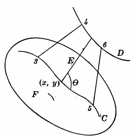
Var Two important auxiliary formulas

Section 2.5 Two important auxiliary formulas

The type of proof used in the preceding section to show that the straight line joining 1 with 2 is shorter than every other admissible arc joining those two points is a very special one, not applicable in general to problems of the calculus of variations whose integrals \(I\) have integrands containing one or both of the variables \(x\) and \(y\) as well as \(y'\text{.}\) It will be well worth while, therefore, to consider a second form of proof which will extend somewhat the results already found for the problem of finding the shortest distance between two points, and which will be applicable not only to the problems of shortest distances considered in this chapter but also to those which we shall study later.

We shall need first of all two special cases of more general formulas which are frequently applied in succeeding pages. Let \(E_{34}\) be a straight-line segment of variable length which moves so that its end-points describe simultaneously the two curves \(C\) and \(D\) shown in Figure 2.5.1, and let the equations of these curves in parametric form be

\begin{align*} (C) \quad x \amp=x_3(t), y=y_3(t), \\ (D) \quad x \amp=x_4(t), y=y_4(t). \end{align*}

The length

\begin{equation*} I=\sqrt{\left(x_{4}-x_{3}\right)^{2}+\left(y_{4}-y_{3}\right)^{2}} \end{equation*}

of the segment \(E_{34}\) has the differential

\begin{equation*} dI=\frac{\left(x_{4}-x_{3}\right)\left(d x_{4}-d x_{3}\right)+\left(y_{4}-y_{3}\right)\left(d y_{4}-d y_{3}\right)}{\sqrt{\left(x_{4}-x_{3}\right)^{2}+\left(y_{4}-y_{3}\right)^{2}}} \end{equation*}

When the notation

\begin{equation*} p=\frac{y_4-y_3}{x_4-x_3} \end{equation*}

is used to denote the slope of the line \(E_{34}\) this result may be expressed in the more convenient formula of the following theorem:

Theorem 2.5.2.

If a straight-line segment \(E_{34}\) moves so that its end-points 3 and 4 describe simultaneously two curves \(C\) and \(D\text{,}\) as shown in Figure 2.5.1, then the length \(I\) of \(E_{34}\) has the differential

\begin{equation} dI\left(E_{34}\right)=\left.\frac{dx+p\,dy}{\sqrt{1+p^{2}}}\right|^4_{3}\label{eqn-dI}\tag{2.5.1} \end{equation}

where the vertical bar indicates that the value of the preceding expression at the point 3 is to be subtracted from its value at the point 4. In this formula the differentials \(dx, dy\) at the points 3 and 4 are those belonging to \(C\) and \(D\text{,}\) while \(p\) is the slope of the segment \(E_{34}\text{.}\)

We shall need frequently to integrate the expression in the second member of (2.5.1) along curves such as \(C\) and \(D\text{.}\) This is evidently justifiable along \(C\text{,}\) for example, since the slope \(p=(y_4-y_3)/(x_4-x_3)\) is a function of \(t\) and since the differentials \(dx, dy\) can be calculated in terms of \(t\) and \(dt\) from the equations of \(C\text{,}\) so that the expression takes the form of a function of \(t\) multiplied by \(dt\text{.}\) The integral \(I^*\) defined by the formula

\begin{equation} I^* = \int \frac{dx+p\,dy}{\sqrt{1+p^{2}}}\label{eqn-i-star}\tag{2.5.2} \end{equation}

will also be well defined along an arbitrary curve \(C\) when \(p\) is a function of \(x\) and \(y\text{,}\) provided that we agree to calculate the value of \(I^*\) by substituting for \(x, y, dx, dy\) the expressions for these variables in terms of \(t\) and \(dt\) obtained from the parametric equations of \(C\text{.}\)

Let \(t_3\) and \(t_5\) be two parameter values which define points 3 and 5 on \(C\text{,}\) and which at the same time define two corresponding points 4 and 6 on \(D\text{,}\) as in Figure 2.5.1. If we integrate the formula (2.5.1) with respect to \(t\) from \(t_3\) to \(t_5\) and use the notation \(I^*\) just introduced for the integral of its second member, we find as a further result:

Theorem 2.5.3.

The difference of the lengths \(I(E_{34})\) and \(I(E_{56})\) of the moving segment in two positions \(E_{34}\) and \(E_{56}\) is given by the formula

\begin{equation} I(E_{56}) - I(E_{34}) = I^*(D_{46}) - I^*(C_{35}).\label{eqn-8}\tag{2.5.3} \end{equation}

This and the formula (2.5.1) are the two important ones for which we have been seeking. It is evident that they will still hold in even simpler form when one of the curves \(C\) or \(D\) degenerates into a point, since along such a degenerate curve the differentials \(dx\) and \(dy\) are zero.

The integrand of the integral \(I^*\) has a simple geometrical interpretation at the points of the curve \(C\) along which it is taken. At the point \((x, y) \)of the curve \(C\) in Figure 2.5.1, for example, the angles between the \(x\)-axis and the tangents to \(C\) and \(E\) have, respectively, the cosines and sines

\begin{equation*} \frac{x^{\prime}}{\sqrt{(x')^2 + (y')^2}}, \frac{y^{\prime}}{\sqrt{(x')^2 + (y')^2}} ; \quad \frac{1}{\sqrt{1+p^{2}}}, \quad \frac{p}{\sqrt{1+p^{2}}} \end{equation*}

Since the angle \(\theta\) between these tangents, and the element of length \(ds\) on \(C\text{,}\) are defined by the equations

\begin{equation} \cos \theta=\frac{x^{\prime}+p y^{\prime}}{\sqrt{\left(1+p^{2}\right)\left((x')^2 + (y')^2\right)}}, \quad ds=\sqrt{(x')^2 + (y')^2}\, dt\label{eqn-9}\tag{2.5.4} \end{equation}

it follows that the integral \(I^*\) can also be expressed in the convenient form

\begin{equation} I^{*}=\int \frac{d x+p\,d y}{\sqrt{1+p^{2}}}=\int \cos \theta\, ds.\label{eqn-10}\tag{2.5.5} \end{equation}