Section1.3Two problems of the calculus of variations which may be simply formulated
When one realizes the difficulty with which the late seventeenth-century school of mathematicians established the first fundamental principles of the calculus and their applications to such elementary problems in maxima and minima as the one which has just been described, it is remarkable that they should have conceived or attempted to solve with their relatively crude analytical machinery the far more difficult maximum and minimum problems of the calculus of variations which were at first proposed. It is an interesting fact that these early problems were not by any means the least complicated ones of the calculus of variations, and we shall do well therefore to introduce ourselves to the subject by looking first at two others which are easier to describe to one who has not already amused himself by browsing in this domain of mathematics.
The simplest of all the problems of the calculus of variations is doubtless that of determining the shortest arc joining two given points. The co-ordinates of these points will always be denoted by \((x_1, y_1)\) and \((x_2, y_2)\) and we may designate the points themselves when convenient simply by the numerals 1 and 2. If the equation of an arc is taken in the form
\begin{equation*}
y=y(x) \quad (x_1\leq x \leq x_2)
\end{equation*}
then the conditions that it shall pass through the two given points are
where in the evaluation of the integral \(y'\) is to be replaced by the derivative \(y'(x)\) of the function \(y(x)\) defining the arc. There is an infinity of curves \(y = y(x)\) joining the points 1 and 2. The problem of finding the shortest one is equivalent analytically to that of finding in the class of functions \(y(x)\) satisfying the conditions (1.3.1) one which makes the integral \(I\) a minimum.
The value of the integral given above clearly depends on what function \(y(x)\) you choose, but will give you a unique output for any function you input. It’s thus an example of a functional -- that is, a function whose inputs are functions and whose outputs are numbers. Using the notation introduced in Activity 2.1.1, we might write that a functional is a function from a class of functions to the real numbers:
Many authors insist on writing functionals with brackets instead of parentheses around their arguments, so you might commonly see someone write something like
Where on earth did that integral come from? Let’s figure it out, because it’s a good example of the slice-approximate-integrate paradigm that guides a lot of the integrals we’ll be writing down in this course, and this integral in particular is one that will come up a lot for us.
Draw yourself a reasonably wiggly function \(y=y(x)\) whose length you’d like to calculate. Label the beginning point \((x_1, y(x_1))\text{,}\) and label the ending point \((x_2, y(x_2))\text{.}\) Draw a few other points on the function at regularly-spaced intervals.
It’s easy to calculate the length of a straight line, so let’s slice the wiggly function into a bunch of pieces and approximate each piece by a straight line. Connect the points you drew in step 1 with straight line segments, and convince yourself that the line segments are a reasonably good wrong answer to the length of the corresponding wiggly piece.
Draw a zoomed-in picture of just one line segment. Pretend that this is the hypotenuse of a right triangle with horizontal and vertical legs. Label each leg as either \(\Delta x\) or \(\Delta y\text{.}\)
So that our expression can be the summand in a Riemann sum, we’d really like it to be of the form (stuff)\(\cdot\Delta x\text{.}\) It’s not in that form yet, so to get closer, multiply \(L_{\textrm{slice}}\) by \(\frac{\Delta x}{\Delta x}\text{.}\) This is legit because it doesn’t change the value of \(L_{\textrm{slice}}.\) Explain why not.
\(\frac{\Delta x}{\Delta x}\) is just a \(1\) with a cheap disguise on, and multiplying by \(1\) doesn’t change anything at all. Multiplying by a fancy \(1\) (as well as adding a fancy \(0\)) is a favorite trick of mathematicians.
Factor the \(\Delta x\) in the denominator into the square root, distribute, and simplify. What happens as \(n\to\infty\text{,}\) or, in other words, as \(\Delta x \to 0?\)
We’ve sliced, we’ve approximated, and now it’s time to integrate. We’ve written down an expression for the length of one slice. Take the Riemann sum of all these slices and let \(n\to\infty\) to obtain an expression for the actual arc length of the wiggly function. Be sure to involve \(x_1\) and \(x_2\text{!}\)
In the more elementary minimum problem of Section 1.2 a function \(f(x)\) is given and a value \(x = a\) is sought for which the corresponding value \(f(a)\) is a minimum. In the shortest-distance problem the integral \(I\) takes the place of \(f(x)\text{,}\) and instead of a value \(x = a\) making \(f(a)\) a minimum we seek to find an arc \(E_{12}\) joining the points 1 and 2 which shall minimize \(I\text{.}\) The analogy between the two problems is more perspicuous if we think of the length \(I\) as a function \(I(E_{12})\) whose value is uniquely determined when the arc \(E_{12}\) is given, just as \(f(x)\) in the former case was a function of the variable \(x\text{.}\)
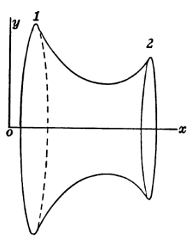
There is a second problem of the calculus of variations, of a geometrical-mechanical type, which the principles of the calculus readily enable us to express also in analytic form. When a wire circle is dipped in a soap solution and withdrawn, a circular disk of soap film bounded by the circle is formed. If a second smaller circle is made to touch this disk and then moved away the two circles will be joined by a surface of film which is a surface of revolution in the particular case when the circles are parallel and have their centers on the same axis perpendicular to their planes. The form of this surface is shown in Figure 2. It is provable by the principles of mechanics, as one may readily surmise intuitively from the elastic properties of a soap film, that the surface of revolution so formed must be one of minimum area, and the problem of determining the shape of the film is equivalent therefore to that of determining such a minimum surface of revolution passing through two circles whose relative positions are supposed to be given as indicated in the figure.
In order to phrase this problem analytically let the common axis of the two circles be taken as the \(x\)-axis, and let the points where the circles intersect an \(xy\)-plane through that axis be 1 and 2. If the meridian curve of the surface in the \(xy\)-plane has an equation \(y=y(x)\) then the calculus formula for the area of the surface is \(2\pi\) times the value of the integral
Aside
\begin{equation*}
I=\int_{x_1}^{x_2} y \sqrt{1+(y')^2}\,dx.
\end{equation*}
The problem of determining the form of the soap film surface between the two circles is analytically that of finding in the class of arcs \(y=y(x)\) whose ends are at the points 1 and 2 one which minimizes the last-written integral \(I\text{.}\)